 The
initial Excel page can be obtained by opening the Excel link located under
start. Depending on your task, your necessities will be laid out as follows:
The
initial Excel page can be obtained by opening the Excel link located under
start. Depending on your task, your necessities will be laid out as follows:
![]() The
initial Excel page can be obtained by opening the Excel link located under
start. Depending on your task, your necessities will be laid out as follows:
The
initial Excel page can be obtained by opening the Excel link located under
start. Depending on your task, your necessities will be laid out as follows:
Home:
Clipboard, Fonts, Alignment, Number, Styles, Cells, Editing
Insert:
Tables, Illustrations, Charts, Links, Text
Page Layouts:
Themes, Page Setup, Scale to Fit, Sheet Options, Arrange
Formulas:
Function Library, Defined Names, Formula Auditing, Calculation
Data:
Get External Data, Connections, Sort & Filter, Data Tools, Outline
Review:
Proofing, Comments, Changes
View:
Workbook Views, Show/Hide, Zoom, Window, Macros
Figure 2: Data entry:
![]()
 Select
the cell that you want your data to appear and begin typing. To enter data into
another cell you can use your arrow keys, your mouse or the tab key.
Select
the cell that you want your data to appear and begin typing. To enter data into
another cell you can use your arrow keys, your mouse or the tab key.
Figure 3: Formatting Cells for Significant Figures:
![]()
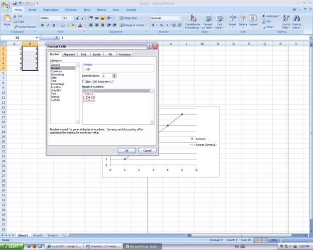 To
set the cells to the correct number of significant figures, right click on the
letter of the column that you want your sig-figs. Go down to the format
cells option and select. You can then go to number and
alter the sig-figs by changing the decimal places.
To
set the cells to the correct number of significant figures, right click on the
letter of the column that you want your sig-figs. Go down to the format
cells option and select. You can then go to number and
alter the sig-figs by changing the decimal places.
Figure 4: Preparing to Graph Data:
![]() To graph data, put
your x-coordinates in the left-hand column and your y-coordinates in the right
hand column as if you were typing a coordinate pair (x,y). After filling in
your data, highlight the data that you want to appear in the graph by selecting
the upper left-hand corner of the first cell to be graphed. Left click and drag
right and down until all cells to be graphed are highlighted. Release the left
mouse button.
To graph data, put
your x-coordinates in the left-hand column and your y-coordinates in the right
hand column as if you were typing a coordinate pair (x,y). After filling in
your data, highlight the data that you want to appear in the graph by selecting
the upper left-hand corner of the first cell to be graphed. Left click and drag
right and down until all cells to be graphed are highlighted. Release the left
mouse button.
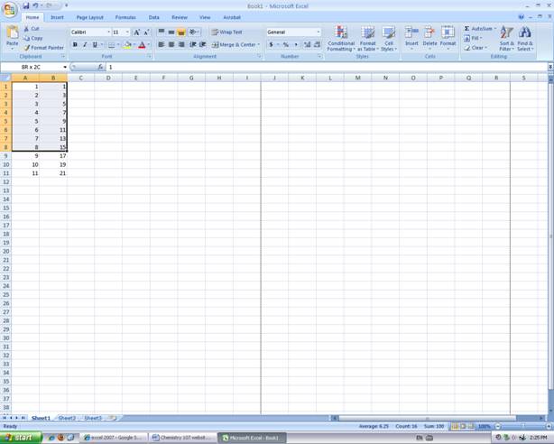
Figure 5: Graphing the Data:
![]() Click insert in the
tool bar and notice the graph options. Under scatter, choose the
option for the XY Scatter.
Click insert in the
tool bar and notice the graph options. Under scatter, choose the
option for the XY Scatter.
Figure 6: Changing Titles and Labels:
![]() Select the chart. Go
to the layout tab and click chart title or
data labels and from there you will be able to alter your titles.
Select the chart. Go
to the layout tab and click chart title or
data labels and from there you will be able to alter your titles.
Figure 7: Adding a Trendline and an Equation to Your Graph:
![]() Under the layout
tab, look to the right of the tool bar and you should see the trendline
option. Select it and go to the bottom of the option list where more
trendline options will be located. Click on it and select your
trendline type which will most likely be the linear trendline. Before exiting
out of the window, you can get your equation by checking on display
equation on chart option located at the bottom of the window.
Under the layout
tab, look to the right of the tool bar and you should see the trendline
option. Select it and go to the bottom of the option list where more
trendline options will be located. Click on it and select your
trendline type which will most likely be the linear trendline. Before exiting
out of the window, you can get your equation by checking on display
equation on chart option located at the bottom of the window.
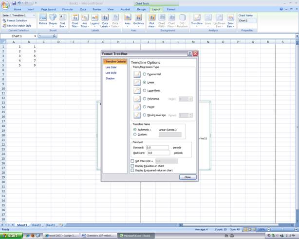
Figure 8-a: Printing Your Graph:
![]()
 If
you simply hit print, your graph may come out on two pages. To prevent this,
simply click the top, left-hand button, go to print preview. This will show you
how your graph will print.
If
you simply hit print, your graph may come out on two pages. To prevent this,
simply click the top, left-hand button, go to print preview. This will show you
how your graph will print.
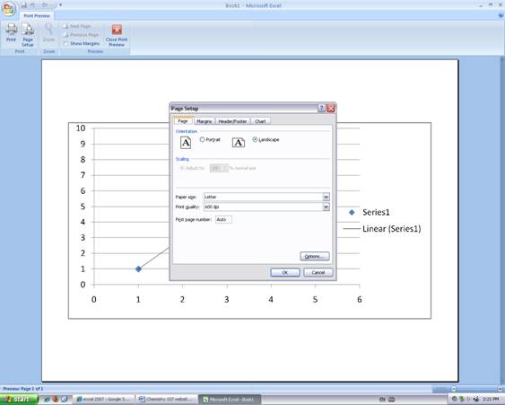
Figure 8-b:
![]() If it needs to be
fixed, locate and click page setup at the top, left-hand side of
the screen. Once that window is open, selecting landscape will fix the problem.
If it needs to be
fixed, locate and click page setup at the top, left-hand side of
the screen. Once that window is open, selecting landscape will fix the problem.
For more information see: http://www.fgcu.edu/support/office2007/Excel/index.asp
Resources:
http://www.fgcu.edu/support/office2007/Excel/index.asp
Kathie A Snyder
Terry L. McAlister
Willie Aiken